Course Navigation
Course Home Expand All

Quantifying Performance Improvement by Fracturing – A Flow Rate Calculator

Real wells, when flowing unrestricted under a constant wellbore pressure, will flow at their maximum rate initially and then uniformly decline in rate with time. Using published equations1Gringarten, A. C., Ramey, H. J., & Raghavan, R. (1972, October). Pressure analysis for fractured wells [Paper presentation]. Fall Meeting of the Society of Petroleum Engineers of AIME, San Antonio, TX, United States. https://doi.org/10.2118/4051-MSwithin the confines of our simplifying assumptions, we have constructed a production rate calculator. In addition to predicting time-dependent radial flow, the calculator predicts production through time for a hydraulic fractured vertical well under the same reservoir conditions.

Results from our flow rate calculator demonstrate the performance capability of hydraulic fracturing in high (100 md) to low (0.1 md) to ultra-low (0.001 md) permeability reservoirs in comparison to radial flow vertical wells. Figures 2.4.1 through 2.4.3 show the rate vs time predictions using the basic reservoir properties already specified for the examples of topic 2.1. The x and y axes in the plots are log-based to better illustrate the time variation and differences between the unfractured and fractured well responses. However, there is an inset in each figure with a linear y-axis to provide additional perspective.

A. High Permeability Conventional Reservoir (k = 100 md)

A reservoir with a 100 md permeability is typically not hydraulically fractured, although there is an exception for wells prone to formation sand production that require gravel packs. For more on this subject, you can follow this deep dive section.

Examining the flow rate results for the fractured and unfractured wells for the case of 100 md (Figure 2.4.1) illustrates why hydraulic fracturing provides limited benefit in this situation. The flow rate at 1 day for the unfractured well is substantial, approximately 5,700 STB/day, very close to the steady state calculation from topic 2.1 (demonstrating the usefulness of the simple analytical equation). The fractured well rate is considerably higher at 21,000 STB/day*This rate is extremely high for a production well, and would exceed the capacity of the typical wellbore tubulars and surface facilities that would be built. Because of these limitations, this rate would likely be unrealized, showing a productivity multiplier of nearly 4. However, the superiority of the fractured well is short-lived, dwindling to J/Jo = 1.4 by the 10 day mark. By 50 days, J/Jo is less than 1.1. These results indicate that for a high permeability well, hydraulic fracturing has limited utility that may not justify the stimulation cost.

Figure 2.4.1: A log-log plot of oil production rate vs time for a fractured and an unfractured (radial flow) vertical well, k = 100 md case. Other simulation parameters include φ = 0.12, μ = 1 cp, ct = 1×10⁻⁵ psi−1, A = 1,742,400 ft2, ΔP = 1,700 psi, h = 50 ft, Bo = 1.3 RB/STB and skin = 0. Pseudo-steady state begins at 0.37 days, which is off the chart to the left. The inset chart is the same data with the y-axis changed to linear instead of log.

B. Low Permeability Unconventional Well Example (k = 0.1 md)

The low permeability case of k = 0.1 md is a more typical hydraulic fracturing candidate (Figure 2.3.3). Initial rates for the fractured and unfractured wells here are much lower than in Figure 2.3.2, in line with the 1,000 times lower permeability, but the productivity advantage of fracturing this well is clearly more significant. Whereas the unfractured well rate at 1 day is only 11 STB/day, the fractured well is producing at 574 STB/day, a J/Jo ~ 50 (meaning the fractured well produces 50 times more than the unfractured well). The rate decline of the fractured well is steeper than that for the unfractured well (which is most clear in the inset chart with a linear y-axis), meaning J/Jo decreases with time, but at 1,000 days J/Jo is still on the order of 10. Beyond 1,000 days, the rates for the two different wells converge more strongly.

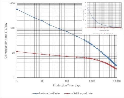
Figure 2.4.2: A log-log plot of oil production rate vs time for a fractured and an unfractured (radial flow) vertical well, k = 0.1 md case. Other simulation parameters include φ = 0.12, μ = 1 cp, ct = 1×10⁻⁵ psi−1, A = 1,742,400 ft2, ΔP = 1,700 psi, h = 50 ft, Bo = 1.3 RB/STB and skin = 0. Pseudo-steady state begins at 372 days. The inset chart is the same data with the y-axis changed to linear instead of log.

C. Ultra-Low Permeability Unconventional Well Example (k = 0.001 md)*This example stretches the applicability of our simple model. One reason is that some researchers question the validity of Darcy’s Law for ultra-low permeability shales. However, the qualitative lessons that can be derived are still worthwhile, even though the quantitative results may be less than realistic

Examining results with a permeability more comparable to a shale, k = 0.001 md (Figure 2.3.4), the 1 day fractured well is at 66 STB/day, 250 times that of the unfractured well. At a year, the J/Jo ratio is still greater than 30. The convergence of rates as each well declines with time is less pronounced than for the 0.1 md case, indicating that a high J/Jo is more persistent. At only a year, the fractured well rate has declined from the initial 66 STB/day, a potential economically viable rate, to only 3 STB/day, which is a condition where abandonment would be considered. But it is important to note that unconventional shale reservoirs are not developed with vertical wells with just one fracture, but instead are drilled with horizontal wells with laterals of 5,000 ft to 15,000 ft in length. These long laterals provide the foundation to place 100 fractures or more flowing to a single well, such that a multi-frac horizontal well will produce significantly more than a single fracture vertical well.

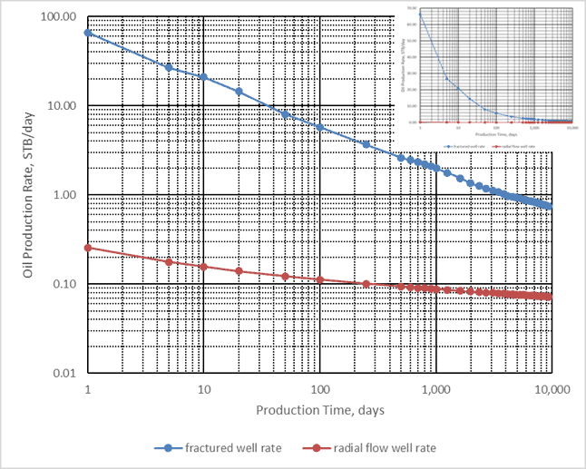
Figure 2.4.3: A log-log plot of oil production rate vs time for a fractured and an unfractured (radial flow) vertical well, k = 0.001 md case. Other simulation parameters include φ = 0.12, μ = 1 cp, ct = 1×10⁻⁵ psi−1, A = 1,742,400 ft2, ΔP = 1,700 psi, h = 50 ft, Bo = 1.3 RB/STB and skin = 0. Pseudo-steady state begins at 37,200 days, which is off the chart to the right. The inset chart is the same data with the y-axis changed to linear instead of log.

Deeper Dive – Link for production rate calculator