Geophysical Techniques
We can start to think of this method by thinking about earthquakes. There are two basic seismic waves that travel through the Earth; longitudinal (P-waves) and shear (S-waves). P waves represent compressional waves of movements (imagine pushing something), and S-waves represent sinusoidal movement (like holding one end of a rope and moving it up and down quickly). There are others, such as Love and Rayleigh waves, but we will only cover the basics here.
Seismometers measure the vertical and horizontal movement generated by an earthquake, and the time at which the P and S waves arrive. This allows us to determine the strength of the earthquake, as measured logarithmically on the Richter scale, and the precise location. P waves and S waves originate at the focus of the earthquake and travel through the Earth’s interior to arrive at seismometers around the world. P-waves travel faster than the S-waves and will arrive first, while the S-wave will arrive at a later time. P-waves and S-waves will also travel at different speeds in different types of rocks. It’s also important to note that S-waves are unable to travel through liquid, and will not travel through the Earth’s outer core.
Let’s think of this with two different layers of the Earth’s crust.
 Reflection seismology uses the principles of seismology, or the propagation of waves through the Earth to estimate the rock properties of subsurface formations.
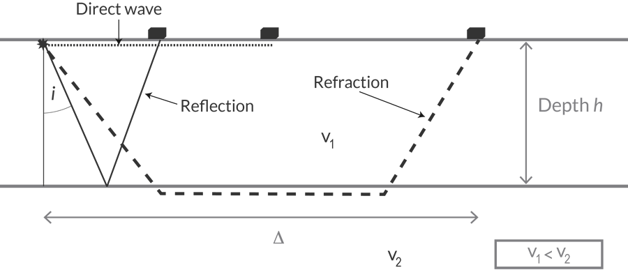
Some seismic wave-producing source, whether it be an explosion, earthquake, or vibration engine (sometimes called a thumper truck) generates waves that are picked up by three separate receivers on Earth’s surface (black boxes). Layer one has a thickness h and a certain velocity, v1. Layer 1 overlies Layer 2, which has a different velocity v2.
We can determine the travel time of the three basic waves, the direct wave, the reflection wave and the refraction wave, as a function of the velocity of the layers and the distance from the source using Snell’s Law:
$$\frac {\sin i_1}{v_1} = \frac {\sin i_2}{v_2}$$
Where v is the velocity of each layer of rock, and i is the incidence angle.
Now we can calculate the travel time for each wave.
First is the direct wave. The direct wave travels with v1 along the surface to the receiver.
$$t_{dir} = \frac {\Delta} {v_1}$$
Now the basics of refraction seismology are the same as for reflection seismology. tdir is the travel time, v1 is the velocity and Δ (“delta”) is the distance traveled.
Calculating the travel time of the refracted wave requires some geometry:
$$t_{refl} = \frac {2} {v_1} \sqrt { (\frac {\Delta} {2})^2 + h^2 }$$
Where h is the thickness of layer 1.
And finally, the reflected wave. This is a bit more complicated because the energy of the wave propagates horizontally in layer 2. So more geometry:
We can see that the emergence angle of the wave is 90 degrees in layer 2, so:
$$ \frac {\sin i_c}{v_1} = \frac {\sin 90^\circ}{v_2} = \frac {1}{v_2} \Rightarrow \sin i_c = \frac {v_1}{v_2}$$
Where ic is the critical angle, in this case 90 degrees.
So the travel time given as a function of distance is
$$t_{refr} = \frac {2h\cos i_c}{v_1} + \frac {\Delta}{v_2} = {t^1}_{refr} + \frac {\Delta}{v_2} $$
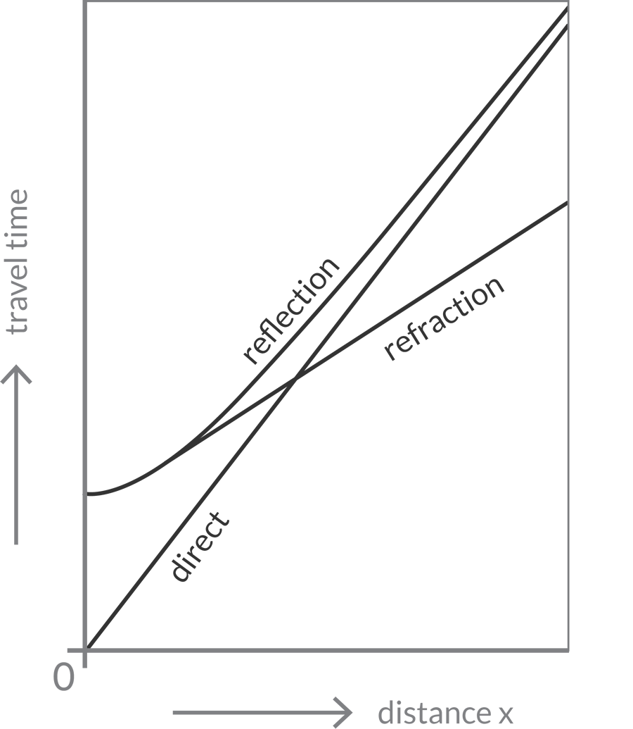
Ultimately we can end up with information like this graph.
Clearly the Earth is composed of many different layers, but we won’t go into that here. A figure like this is important because it allows scientists to get the best data out of seismic surveys. Seismic surveys use reflection seismology, rather than refraction seismology, but the principles are basically the same. Basically the difference between the two is that when we use refraction seismic we need to measure a greater distance at the Earth’s surface with respect to the depth of interest.
In reflection seismology, we are interested in relatively small offsets, and therefore need a shorter distance with respect to the depth of interest.
So to image the subsurface, scientists will generate an artificial earthquake and measure the travel times of the waves. The primary goal is to identify reflectors, or the surface where the waves bounce back.
We should also just briefly chat about acoustic impedence which is basically the product of the density of the rock and the wave velocity. This matters because we will see differences in amplitudes at layer boundaries. When a seismic wave encounters a layer boundary, some the energy bounces back while some of it will be transmitted to the next layer. So the larger the contrast between the two different layers, the larger the amplitude of the wave that was bounced back.
Tying this information with well information allows us to map and interpret potential hydrocarbon reserves.
Gravity Survey
Gravity surveys are based on the fundamentals that all things have a gravitational attraction. Gravitational attraction is proportional to mass; the denser something is, the larger the gravity.
These basics allows scientists to determine variations in the subsurface of the Earth. For field surveys we will usually indirectly measure gravity, and measure the relative gravity. This means that we don’t get an absolute measurement, but get an idea on how gravity changes from place to place.
Seems relatively simple but several corrections need to be made to results since gravity is affected by other things besides calibration and drift. One is altitude, or the height of the ground measurement. To correct for these variations we also need height measurements at each location. The other is that gravity changes at different latitudes.
Magnetic Surveys
Magnetic surveys measure small variations in the Earth’s magnetic field. The Earth possess a magnetic field due to convection of the liquid iron rich outer core. You can think of a bar magnet at the center of the earth with field lines that exit the South pole and enter at the North pole. Magnetic north and south poles are subparallel to the geographic poles. The intensity of the Earth’s magnetic field also varies from the equator to the poles, and is measured in nanoteslas (nT).
Most materials exhibit an induced magnetic field basically due to the behavior of the material when the material is influenced by Earth’s stronger magnetic field. This induced magnetic field refers to the magnetic field on a material where the ambient field is enhanced because the material itself behaves like a magnet. This field is proportional to the intensity of the ambient field and the ability of the new magnetic material to enhance the ambient field is called magnetic susceptibility:
$$ I = kF $$
k = magnetic susceptibility, F = field intensity (Tesla), and I = induced magnetization
What causes magnetic susceptibility?
At the atomic level, magnetic materials have a net magnetic moment. This is because of the spin of electrons, the rotation of electrons around the nucleus, and the number of electrons in each shell.
There are three types of magnetic materials.
Diamagnetic materials are those that in the presence of an external field oppose the external field. Electron shells are filled and there is no net magnetic moment.
Paramagnetic materials are those that have unpaired electrons in incomplete shells, and the magnetic moment is not coupled with other atoms, so each one behaves independently. These are weakly magnetic materials.
Ferromagnetic materials are those that have unpaired electrons in incomplete shells and the magnetic moment is coupled with other atoms such that they all become parallel to one another. These materials are magnetic, even in the absence of a magnetic field (i.e. magnets).
K is generally much less than 1, except for magnetite. Iron steel and iron alloys have susceptibilities several orders of magnitude greater than magnetite. We may not be see significant contrasts between sedimentary rocks, but we can easily use magnetic surveys to map different geologic units where there are units that are iron rich.
| Rock Type | Susceptibility (k) |
|---|---|
| Altered ultra basics | 10-4 to 10-2 |
| Basalt | 10-4 |
| Gabbro | 10-4 to 10-3 |
| Granite | 10-5 to 10-3 |
| Andesite | 10-4 |
| Rhyolite | 10-5 to 10-4 |
| Metamorphic rocks | 10-4 to 10-6 |
| Most sedimentary rocks | 10-6 to 10-5 |
| Limestone and chert | 10-6 |
| Shale | 10-5 to 10-4 |